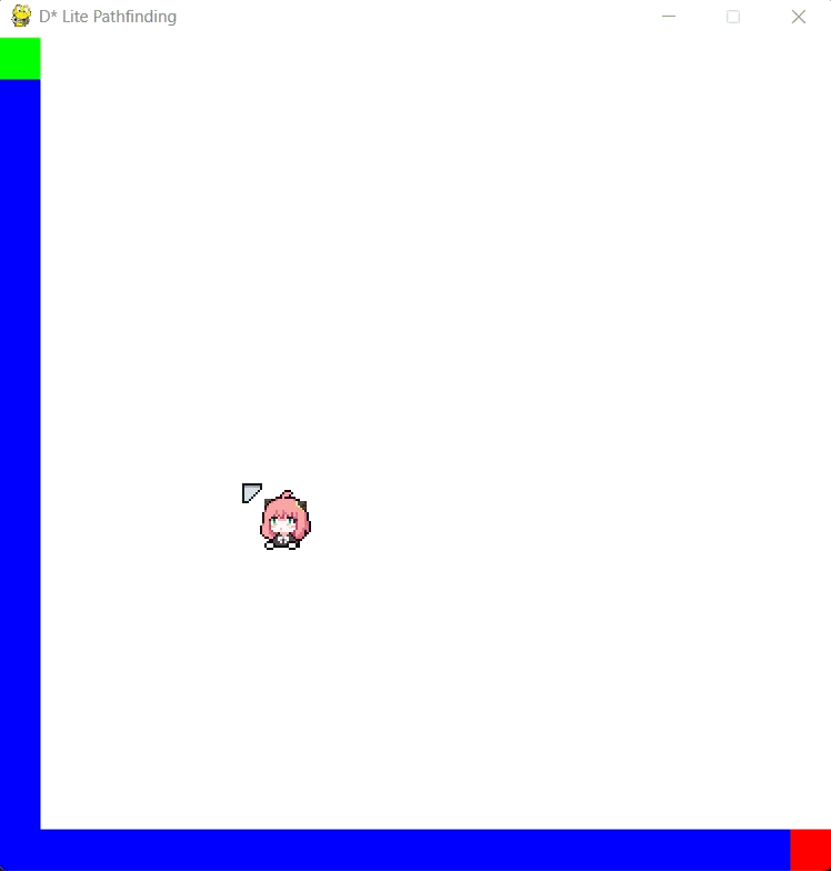
D* Lite in action at 20x20 grid
Introduction
D* (star) Lite Pathfinding algorithm, or any path finding algorithm in short, is a procedure used to find the optimal path between two points in a given environment. It could be the way to find the shortest path between this road to that road, or the path that shown in the Google Map between a location to a location.
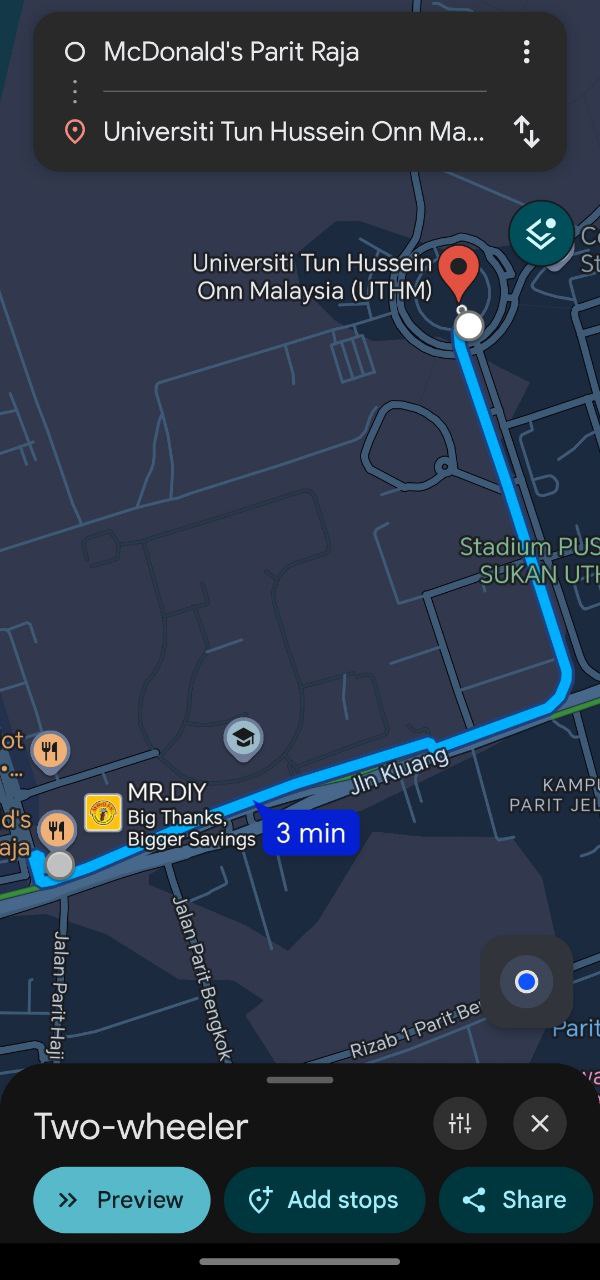
Shortest Path from McDonald's Parit Raja to UTHM.
There are numerous well-known path finding algorithm, which includes A* algorithm, Dijkstra’s algorithm, and also the D* algorithm. I believe there are numerous websites who do the explanation of each algorithm, but in short, each algorithm serves it’s own purpose.
In the nutshell, Dijkstra algorithm did not using heuristic function, which it is not optimised for dynamic used case. Both A-star and D-star do use heuristic function but A-star are not highly efficient compare to D-star in terms of dynamic environment. There are 3 varients of D-star but I am here only using the D-star lite algorithm as D-star lite is more simplified and more efficient in robotic world and low powered device.
Note: You could refer this A-star vs Dijkstra Algorithms Pathfinding Visualisation from @Borington-Youtube
First Part: D* Lite Algorithm Itself
I refer the works from @Sollimann/Dstar-lite-pathplanner, @SebLague/Pathfinding, and Sebastian Lague A* Pathfinding as reference and starting point to have better understanding of how heuristic function esentially work and how D-star lite algorithm behaving.
In short, D-star lite works in 3 steps:
- We assign a g value (cost from goal) and rhs value (or we call one-step ahead (no jojo reference)) for every single cell exist in the grid.
- Then we maintain a priority queue U to process the most promising cell first, so you may see like a wave from start to end during calculation.
- We only need to recalculate the path as needed.
Step 1: Initialisation
self.g = {}
self.rhs = {}
self.U = []
self.U_set = {}    #Have a quick view what's inside U
self.km = 0  #Biasing
So each grid cell get’s 2 value, g and rhs. And each cell’s g represent current cost from start to s. Then the cell’s rhs is one step ahead of what g[s] should be. Therefore initially all are having inf value except rhs[goal] = 0 since we moving backward from goal.
Step 2: Get the priority
def calculate_key(self, s):
 return (min(g[s], rhs[s]) + heuristic(start, s) + km, min(g[s], rhs[s]))
This is how we compare the priority in the heap, we get the estimation of the cost to reach s plus heuristic function (or known as Manhattan distance) and sum with bias of km.
Step 3: The core part of D-star lite
 def update_vertex(self, s):
        if s != self.goal:
            self.rhs[s] = min(self.cost(s, s_prime) + self.g[s_prime] for s_prime in self.get_neighbors(s))

        if s in self.U_set:
            self.U_set.pop(s, None)

        if self.g[s] != self.rhs[s]:
            self.insert(s, self.calculate_key(s))
This is the core of the D-star lite, which enable the functionality of “being dynamic”. There are 3 cases for the update_vertex():
- Case for s != self.goal
In D-star lite, the rhs value of goal node always fixed to 0. We only need to trigger this condition if s is not the goal node and update the rhs value. We update the rhs value of cell s by first checking all neighbors of s (we denote as s_prime), compute each cost of s to s_prime + g[s_prime], and we get the minimum of cost to real the goal via ONE neighbor.
- Case for s in self.U_set
We check if s is already in the priority queue U, then we remove the old entry of s by remove from U_set (dictionary of U), which avoid duplicates in priority queue by tracking which nodes are there.
- Case for self.g[s] != self.rhs[s]
The core idea of dynamically. When current cost g[s] is differ from expected best cost rhs[s], then something wrong somewhere. So the node s is become inconsistent due to something has changed, and should be reprocess by put it back to priority queue U.
Step 4: Compute the shortest path
 def compute_shortest_path(self):
        while self.U and (self.U[0][0] < self.calculate_key(self.start) or self.rhs[self.start] != self.g[self.start]):
            k_old, u = heapq.heappop(self.U)

            if self.U_set.get(u) == k_old:
                self.U_set.pop(u, None)
            else:
                continue

            if self.g[u] > self.rhs[u]:
                self.g[u] = self.rhs[u]
            else:
                self.g[u] = float('inf')
                self.update_vertex(u)

            for neighbor in self.get_neighbors(u):
                self.update_vertex(neighbor)
We first ensure the compute shortest path always working only when there are nodes in the priority queue U and either top node in the queue has a smaller key than current key of the start node (better key can use), or the start node is different (g != rhs).
Then, we take the node u with lowest key out of the queue and remove duplicates. If g>rhs, we set it to correct value of rhs which has valid path to goal, else we reset g to inf and fix the path again (obstacle added). And we update all the u’s neighbors.
So the loop only stop only and only when the queue is empty or the start’s g and rhs are consistent and no better node exists in the grid.
Step 5: The homerun: Trace the path
def get_path(self):
        path = []
        s = self.start

        if self.g[self.start] == float('inf'):
            return []

        visited = set()
        while s != self.goal:
            path.append(s)
            visited.add(s)

            neighbors = self.get_neighbors(s)
            # Filter out visited neighbors and obstacles
            neighbors = [n for n in neighbors if self.grid[n[0]][n[1]] != 1 and n not in visited]

            if not neighbors:
                return []

            # Find neighbor with smallest g-value
            s_next = min(neighbors, key=lambda s_prime: self.g.get(s_prime, float('inf')))

            if self.g.get(s_next, float('inf')) == float('inf'):
                return []

            s = s_next

        path.append(self.goal)
        return path
In short, we first check if cost of start is inf, meaning no path exist in the grid. Then we keep adding current node to the path and mark as visited until reach the goal. We have to set filters for obstacle which denote as not self.grid[n[0]][n[1]] == 1 and n not in visited. Note: if best neighbor has infinite cost, we are trapped. Note: Keep finding until we reach the end, then we append in path().
Second Part: Python Window Interaction
Esentially, the core part of the algorithm is done, but we have to try it out and make the obstacle dynamic by ourselves right? :P Yep, we are using pygame as the interactive window for the D-star Lite.
Step 1: Initialisation and Display Setup
# Pygame Preconfig
grid_size = int(input("Enter grid size (nxn configuration) : "))
display_size = 800 # max window dimension (width and height)
cell_size = max(4, display_size // grid_size)
window_size = display_size

start = (0, 0) # Green
goal = (grid_size - 1, grid_size - 1) # Red

grid = np.zeros((grid_size, grid_size), dtype=int)

# Pygame init
pygame.init()
win = pygame.display.set_mode((display_size, display_size))
pygame.display.set_caption("D* Lite Pathfinding")
In short, we ask the user the desired grid size with integers. Then we adjust the cell_suze for each cell to ensure all cells can fit inside display_size. We define the window_size as the display_size. Then we define the start and goal point with coordinates preset, and the colors of course. We initialise the grid with zeros as for ones, here indicate as obstacle (with color of 0,0,0).
Step 2: Draw for me
def draw(grid, path, start, goal):
    #... Color settings for start, goal, obstacles
    #The core part
    # Upscale with np.kron
    scale = cell_size
    img = np.kron(colors, np.ones((scale, scale, 1), dtype=np.uint8))

    surf = pygame.surfarray.make_surface(np.transpose(img, (1, 0, 2)))  # transpose for pygame axis
    scaled = pygame.transform.smoothscale(surf, (display_size, display_size))
    win.blit(scaled, (0, 0))
    pygame.display.update()
We use np.kron to scale up the small grid images and transpose it since pygame.surfarray.make_surface() expect (width, height) not (row, col). After that we scale up small surf to fit full display of display_size by using smoothscale() which using anti-aliasing. Then, we draw a “blits”, which is the scaled images onto Pygame windows at pos 0,0. We update it by calling pygame.display.update(), which esentially abit how GPU works :P
Step 3: Interactions
# Initial path
dstar = DStarLite(grid, start, goal)
path = dstar.get_path()

# Main loop
running = True
while running:
    draw(grid, path, start, goal)
    for event in pygame.event.get():
        if event.type == pygame.QUIT:
            running = False

    mouse_buttons = pygame.mouse.get_pressed()
    if any(mouse_buttons):
        x, y = pygame.mouse.get_pos()
        if x >= window_size or y >= window_size:
            continue  # out of bounds

        grid_x, grid_y = y // cell_size, x // cell_size
        if (grid_x, grid_y) in [start, goal]:
            continue

        if mouse_buttons[0]:  # left-click: add
            if grid[grid_x][grid_y] != 1:
                grid[grid_x][grid_y] = 1
                #... do something

        elif mouse_buttons[2]:  # right-click: remove
            if grid[grid_x][grid_y] != 0:
                grid[grid_x][grid_y] = 0
                #... do something
After spun up, we first initialize the path computation function and the entire GUI function works in the while loop, where for left click in the grid turn the grid to =1 , which adding obstacle (black), and right click in the grid turn the grid to = 0, which remove obstacle (white).
Third Part: Metric Performance Measrument
In this case, I notice some pattern when doing some simulations, so I tried to include an option for metric performance measurement.
Step 1: Setup of the measurements.
import matplotlib.pyplot as plt

# Performance Matrix (Can be Commented Out)
metrics = [] #tuples: (obstacle_count, path_length, time_ms)
...
if mouse_buttons[0]:  # left-click: add
            if grid[grid_x][grid_y] != 1:
                grid[grid_x][grid_y] = 1
                t0 = time.time()
                dstar = DStarLite(grid, start, goal)
                path = dstar.get_path()
                elapsed_ms = (time.time() - t0) * 1000
                obstacle_count = np.sum(grid == 1)
                path_length = len(path)
                metrics.append((obstacle_count, path_length, elapsed_ms))
                print(f"Recalculated in {elapsed_ms:.2f} ms, Obstacles: {obstacle_count}, Path Length: {path_length}")

        elif mouse_buttons[2]:  # right-click: remove
            if grid[grid_x][grid_y] != 0:
                grid[grid_x][grid_y] = 0
                t0 = time.time()
                dstar = DStarLite(grid, start, goal)
                path = dstar.get_path()
                elapsed_ms = (time.time() - t0) * 1000
                obstacle_count = np.sum(grid == 1)
                path_length = len(path)
                metrics.append((obstacle_count, path_length, elapsed_ms))
                print(f"Recalculated in {elapsed_ms:.2f} ms, Obstacles: {obstacle_count}, Path Length: {path_length}")
In this case, I need to find the relationship between the time taken to calculate the path and the number of obstacle and also the relationship of number of obstacle added and length of shortest path. Firstly, I have to setup the way to record the parameters by making the 3 parameters into 1 tuple. Before doing that, I need to “probe” the parameters by placing the measurements inside every mouse click event.
Step 2: Plotting Graph
pygame.quit()
# After exit, compile into performance matrix
if metrics:
    # Extract data
    obs, lengths, times = zip(*metrics)

    # Plot
    plt.figure(figsize=(10, 5))

    plt.subplot(1, 2, 1)
    plt.plot(obs, times, 'bo-')
    plt.xlabel("Number of Obstacles")
    plt.ylabel("Recalculation Time (ms)")
    plt.title("Time vs Obstacle Count")

    plt.subplot(1, 2, 2)
    plt.plot(obs, lengths, 'go-')
    plt.xlabel("Number of Obstacles")
    plt.ylabel("Path Length")
    plt.title("Path Length vs Obstacle Count")

    plt.tight_layout()
    plt.show()
The plotting only get triggered once we close the pygame window, indicating we are done for the simulation. I used the zip() function to make the 3 parameters tuple. Then, I plot the 2 graphs in the same window using subplot() function. Which it looks exactly like MATLAB code.
Result and Issues
The gif animation of one of the simulations.
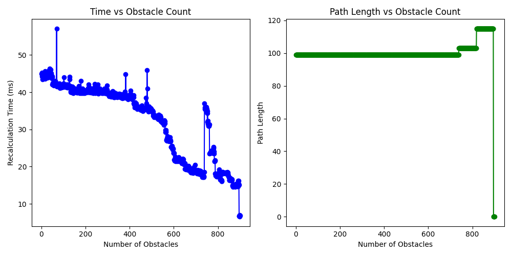
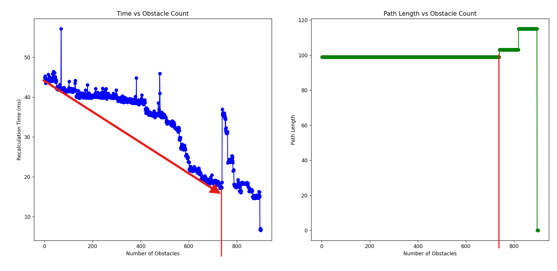
The result of the graph for grid size of 50*50, up to 900 obstacles placed.
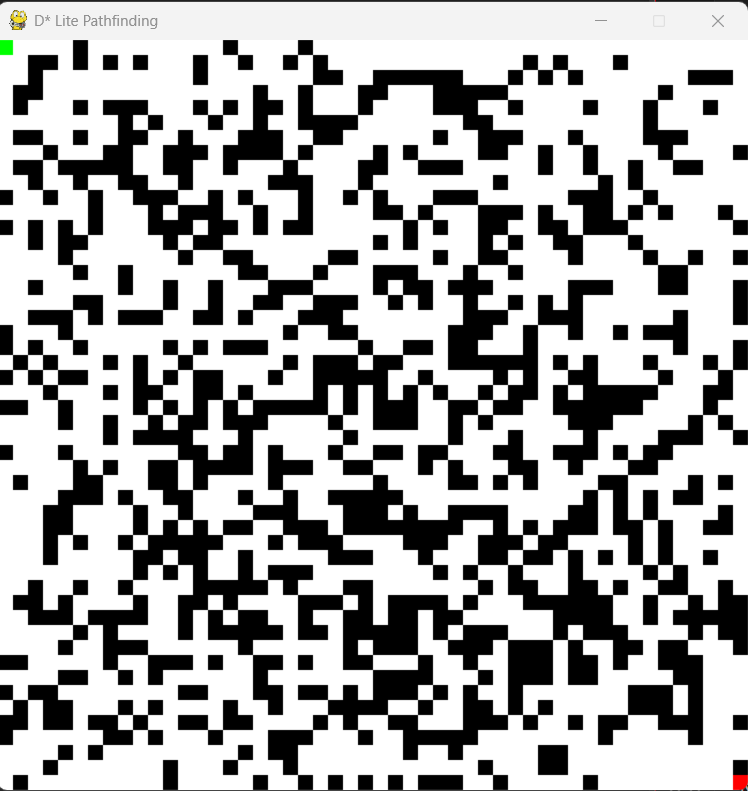
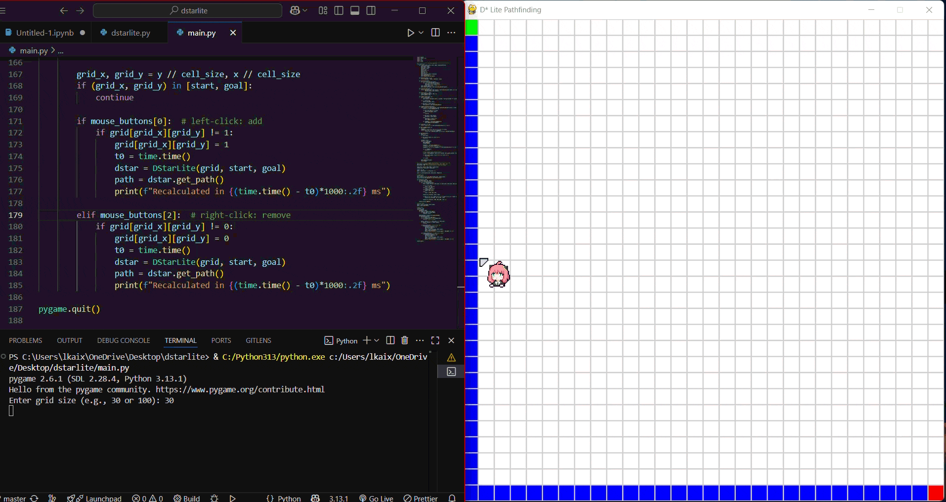
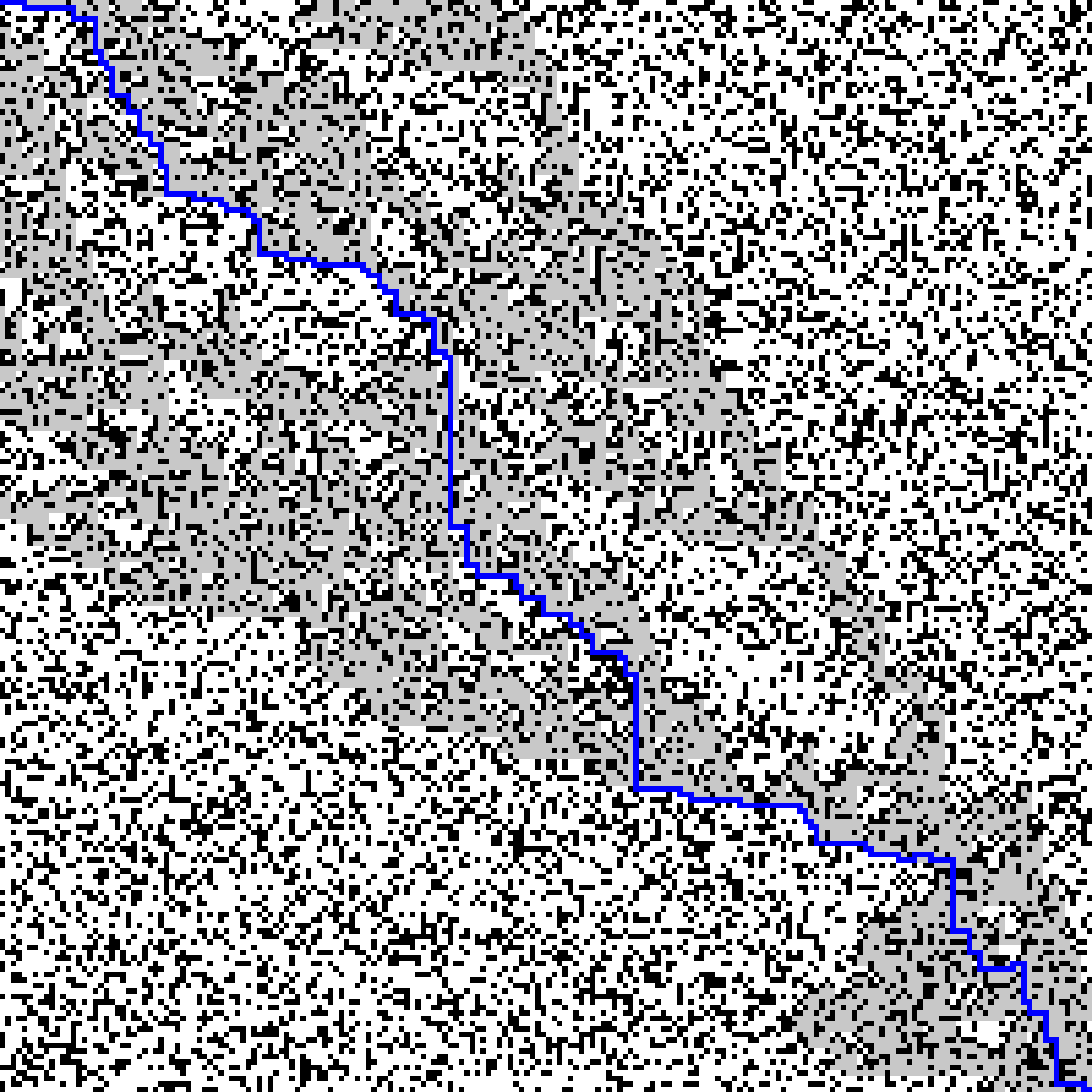
The grid used for the simulation for grid size of 50x50 during 900th obstacle.
Text Log:
Recalculated in 16.20 ms, Obstacles: 894, Path Length: 115
Recalculated in 15.11 ms, Obstacles: 895, Path Length: 115
Recalculated in 6.69 ms, Obstacles: 896, Path Length: 0
Recalculated in 6.69 ms, Obstacles: 897, Path Length: 0
At 896th obstacle, there are no possible path to the goal, therefore the path length = 0. But the time of recalculation indicating the path atleast travelled outside of the start.
First observation: Based on:
Recalculated in 18.58 ms, Obstacles: 738, Path Length: 99
Recalculated in 36.93 ms, Obstacles: 739, Path Length: 103
First observation with using arrow as the overall trend.
Conclusion: If the number of shortest path remain the same even increases in number of obstacle, the calculation time will eventually decrease as less space search required. Therefore, it causing a decrease trend of recalculation time.
Second observation:
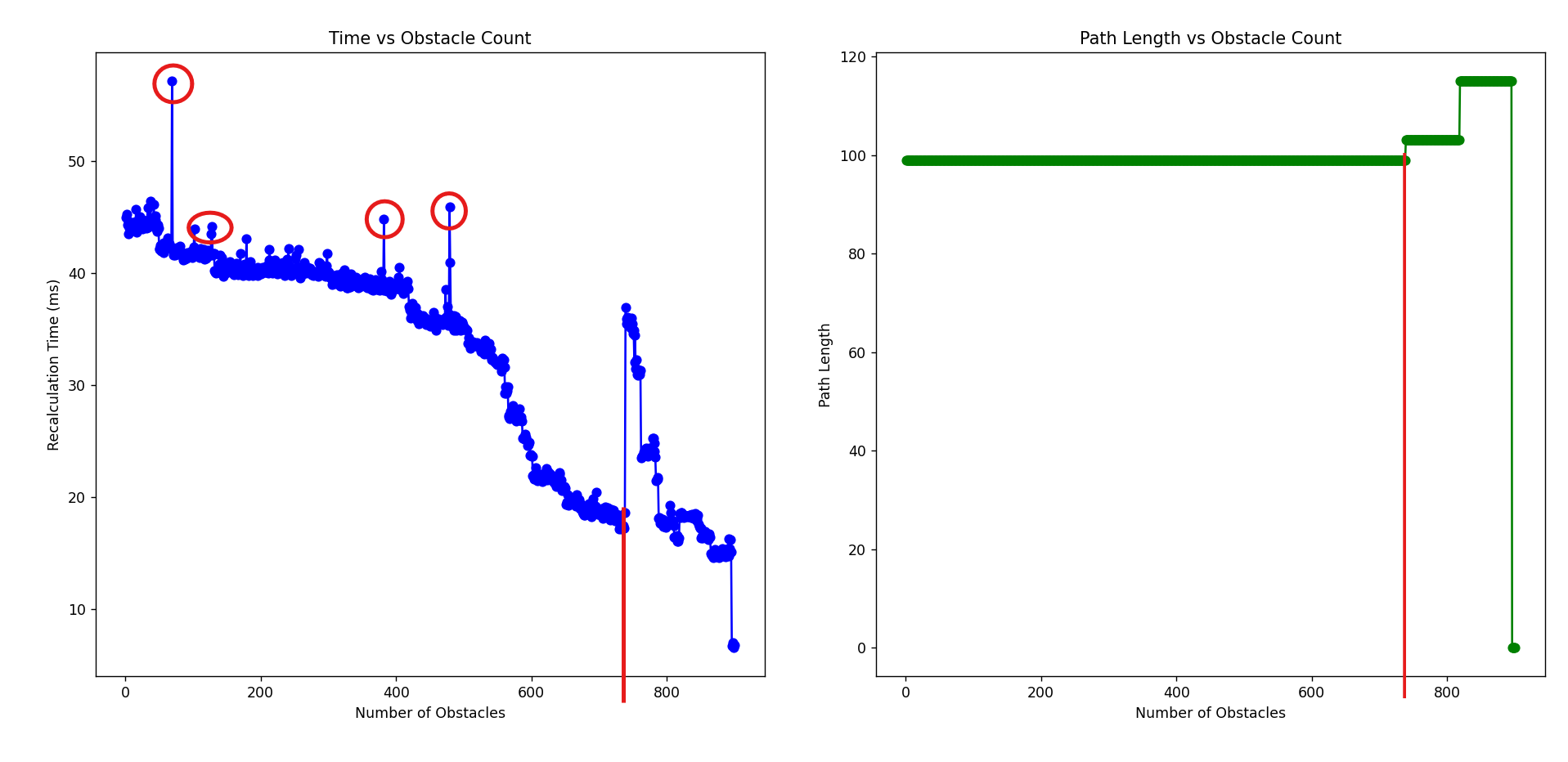
Second observation with high outliers at same number of cells to reach shortest path.
Conclusion: The spike generated at a decreasing trend indicating the current shortest path was obstructed by new obstacle, and required more indexing to recalculate the path, although it still remain the same path length, but it can be different path.
Third observation:
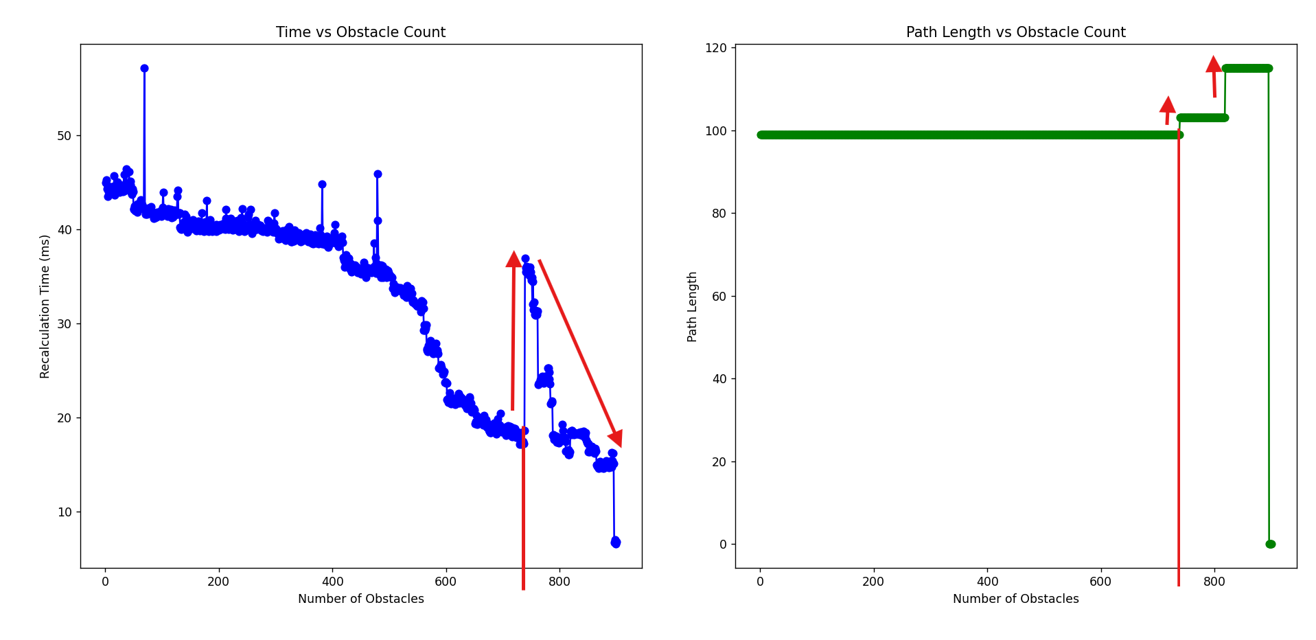
Third observation with opposite trend between 2 graphs.
Conclusion 1: As there is changes of the shortest path length, a new overall recalculation is needed, therefore it spikes up from around 20ms to near 40ms, but the changes is insignifant as there is less search area at placement of 739th obstacle. Conclusion 2: The anomaly of the trend is differ at path length increase from 103 to 115 cells can be explain as even lesser search area.
The issue Since we are using pygame as GUI, therefore the performance issue become a big deal at greater grid size, lets say 200x200. We are starting to get Second per Frame instead of Frames per second.
Recalculated in 756.48 ms, Obstacles: 37, Path Length: 399
Recalculated in 763.96 ms, Obstacles: 38, Path Length: 399
Recalculated in 750.94 ms, Obstacles: 39, Path Length: 399
Which without the GUI, we use randomisation of obstacle placement at same grid size with probability of 30% being obstacle for each cell, which it took 237ms to complete it, here is the result:
200x200 grid in 0.2s? COOL
Conclusion
In short, D-starlite cool. Pygame, cool in some way. Perhaps i am not good at optimizing the GUI :P
Next step
Could it be… interact with ROS2? Call it as node? Made my own robots? And help me buy food? That would be awesome.
Note: Special thanks to the resources, you guys the best Note: Of course, you reached the end of the page, or is it?
layout: post title: “D* (Star) lite algorithm Implementation Using Python” date: 2025-07-16 —
D* Lite in action at 20x20 grid
Introduction
D* (star) Lite Pathfinding algorithm, or any path finding algorithm in short, is a procedure used to find the optimal path between two points in a given environment. It could be the way to find the shortest path between this road to that road, or the path that shown in the Google Map between a location to a location.
Shortest Path from McDonald's Parit Raja to UTHM.
There are numerous well-known path finding algorithm, which includes A* algorithm, Dijkstra’s algorithm, and also the D* algorithm. I believe there are numerous websites who do the explanation of each algorithm, but in short, each algorithm serves it’s own purpose.
In the nutshell, Dijkstra algorithm did not using heuristic function, which it is not optimised for dynamic used case. Both A-star and D-star do use heuristic function but A-star are not highly efficient compare to D-star in terms of dynamic environment. There are 3 varients of D-star but I am here only using the D-star lite algorithm as D-star lite is more simplified and more efficient in robotic world and low powered device.
Note: You could refer this A-star vs Dijkstra Algorithms Pathfinding Visualisation from @Borington-Youtube
First Part: D* Lite Algorithm Itself
I refer the works from @Sollimann/Dstar-lite-pathplanner, @SebLague/Pathfinding, and Sebastian Lague A* Pathfinding as reference and starting point to have better understanding of how heuristic function esentially work and how D-star lite algorithm behaving.
In short, D-star lite works in 3 steps:
- We assign a g value (cost from goal) and rhs value (or we call one-step ahead (no jojo reference)) for every single cell exist in the grid.
- Then we maintain a priority queue U to process the most promising cell first, so you may see like a wave from start to end during calculation.
- We only need to recalculate the path as needed.
Step 1: Initialisation
self.g = {}
self.rhs = {}
self.U = []
self.U_set = {}    #Have a quick view what's inside U
self.km = 0  #Biasing
So each grid cell get’s 2 value, g and rhs. And each cell’s g represent current cost from start to s. Then the cell’s rhs is one step ahead of what g[s] should be. Therefore initially all are having inf value except rhs[goal] = 0 since we moving backward from goal.
Step 2: Get the priority
def calculate_key(self, s):
 return (min(g[s], rhs[s]) + heuristic(start, s) + km, min(g[s], rhs[s]))
This is how we compare the priority in the heap, we get the estimation of the cost to reach s plus heuristic function (or known as Manhattan distance) and sum with bias of km.
Step 3: The core part of D-star lite
 def update_vertex(self, s):
        if s != self.goal:
            self.rhs[s] = min(self.cost(s, s_prime) + self.g[s_prime] for s_prime in self.get_neighbors(s))

        if s in self.U_set:
            self.U_set.pop(s, None)

        if self.g[s] != self.rhs[s]:
            self.insert(s, self.calculate_key(s))
This is the core of the D-star lite, which enable the functionality of “being dynamic”. There are 3 cases for the update_vertex():
- Case for s != self.goal
In D-star lite, the rhs value of goal node always fixed to 0. We only need to trigger this condition if s is not the goal node and update the rhs value. We update the rhs value of cell s by first checking all neighbors of s (we denote as s_prime), compute each cost of s to s_prime + g[s_prime], and we get the minimum of cost to real the goal via ONE neighbor.
- Case for s in self.U_set
We check if s is already in the priority queue U, then we remove the old entry of s by remove from U_set (dictionary of U), which avoid duplicates in priority queue by tracking which nodes are there.
- Case for self.g[s] != self.rhs[s]
The core idea of dynamically. When current cost g[s] is differ from expected best cost rhs[s], then something wrong somewhere. So the node s is become inconsistent due to something has changed, and should be reprocess by put it back to priority queue U.
Step 4: Compute the shortest path
 def compute_shortest_path(self):
        while self.U and (self.U[0][0] < self.calculate_key(self.start) or self.rhs[self.start] != self.g[self.start]):
            k_old, u = heapq.heappop(self.U)

            if self.U_set.get(u) == k_old:
                self.U_set.pop(u, None)
            else:
                continue

            if self.g[u] > self.rhs[u]:
                self.g[u] = self.rhs[u]
            else:
                self.g[u] = float('inf')
                self.update_vertex(u)

            for neighbor in self.get_neighbors(u):
                self.update_vertex(neighbor)
We first ensure the compute shortest path always working only when there are nodes in the priority queue U and either top node in the queue has a smaller key than current key of the start node (better key can use), or the start node is different (g != rhs).
Then, we take the node u with lowest key out of the queue and remove duplicates. If g>rhs, we set it to correct value of rhs which has valid path to goal, else we reset g to inf and fix the path again (obstacle added). And we update all the u’s neighbors.
So the loop only stop only and only when the queue is empty or the start’s g and rhs are consistent and no better node exists in the grid.
Step 5: The homerun: Trace the path
def get_path(self):
        path = []
        s = self.start

        if self.g[self.start] == float('inf'):
            return []

        visited = set()
        while s != self.goal:
            path.append(s)
            visited.add(s)

            neighbors = self.get_neighbors(s)
            # Filter out visited neighbors and obstacles
            neighbors = [n for n in neighbors if self.grid[n[0]][n[1]] != 1 and n not in visited]

            if not neighbors:
                return []

            # Find neighbor with smallest g-value
            s_next = min(neighbors, key=lambda s_prime: self.g.get(s_prime, float('inf')))

            if self.g.get(s_next, float('inf')) == float('inf'):
                return []

            s = s_next

        path.append(self.goal)
        return path
In short, we first check if cost of start is inf, meaning no path exist in the grid. Then we keep adding current node to the path and mark as visited until reach the goal. We have to set filters for obstacle which denote as not self.grid[n[0]][n[1]] == 1 and n not in visited. Note: if best neighbor has infinite cost, we are trapped. Note: Keep finding until we reach the end, then we append in path().
Second Part: Python Window Interaction
Esentially, the core part of the algorithm is done, but we have to try it out and make the obstacle dynamic by ourselves right? :P Yep, we are using pygame as the interactive window for the D-star Lite.
Step 1: Initialisation and Display Setup
# Pygame Preconfig
grid_size = int(input("Enter grid size (nxn configuration) : "))
display_size = 800 # max window dimension (width and height)
cell_size = max(4, display_size // grid_size)
window_size = display_size

start = (0, 0) # Green
goal = (grid_size - 1, grid_size - 1) # Red

grid = np.zeros((grid_size, grid_size), dtype=int)

# Pygame init
pygame.init()
win = pygame.display.set_mode((display_size, display_size))
pygame.display.set_caption("D* Lite Pathfinding")
In short, we ask the user the desired grid size with integers. Then we adjust the cell_suze for each cell to ensure all cells can fit inside display_size. We define the window_size as the display_size. Then we define the start and goal point with coordinates preset, and the colors of course. We initialise the grid with zeros as for ones, here indicate as obstacle (with color of 0,0,0).
Step 2: Draw for me
def draw(grid, path, start, goal):
    #... Color settings for start, goal, obstacles
    #The core part
    # Upscale with np.kron
    scale = cell_size
    img = np.kron(colors, np.ones((scale, scale, 1), dtype=np.uint8))

    surf = pygame.surfarray.make_surface(np.transpose(img, (1, 0, 2)))  # transpose for pygame axis
    scaled = pygame.transform.smoothscale(surf, (display_size, display_size))
    win.blit(scaled, (0, 0))
    pygame.display.update()
We use np.kron to scale up the small grid images and transpose it since pygame.surfarray.make_surface() expect (width, height) not (row, col). After that we scale up small surf to fit full display of display_size by using smoothscale() which using anti-aliasing. Then, we draw a “blits”, which is the scaled images onto Pygame windows at pos 0,0. We update it by calling pygame.display.update(), which esentially abit how GPU works :P
Step 3: Interactions
# Initial path
dstar = DStarLite(grid, start, goal)
path = dstar.get_path()

# Main loop
running = True
while running:
    draw(grid, path, start, goal)
    for event in pygame.event.get():
        if event.type == pygame.QUIT:
            running = False

    mouse_buttons = pygame.mouse.get_pressed()
    if any(mouse_buttons):
        x, y = pygame.mouse.get_pos()
        if x >= window_size or y >= window_size:
            continue  # out of bounds

        grid_x, grid_y = y // cell_size, x // cell_size
        if (grid_x, grid_y) in [start, goal]:
            continue

        if mouse_buttons[0]:  # left-click: add
            if grid[grid_x][grid_y] != 1:
                grid[grid_x][grid_y] = 1
                #... do something

        elif mouse_buttons[2]:  # right-click: remove
            if grid[grid_x][grid_y] != 0:
                grid[grid_x][grid_y] = 0
                #... do something
After spun up, we first initialize the path computation function and the entire GUI function works in the while loop, where for left click in the grid turn the grid to =1 , which adding obstacle (black), and right click in the grid turn the grid to = 0, which remove obstacle (white).
Third Part: Metric Performance Measrument
In this case, I notice some pattern when doing some simulations, so I tried to include an option for metric performance measurement.
Step 1: Setup of the measurements.
import matplotlib.pyplot as plt

# Performance Matrix (Can be Commented Out)
metrics = [] #tuples: (obstacle_count, path_length, time_ms)
...
if mouse_buttons[0]:  # left-click: add
            if grid[grid_x][grid_y] != 1:
                grid[grid_x][grid_y] = 1
                t0 = time.time()
                dstar = DStarLite(grid, start, goal)
                path = dstar.get_path()
                elapsed_ms = (time.time() - t0) * 1000
                obstacle_count = np.sum(grid == 1)
                path_length = len(path)
                metrics.append((obstacle_count, path_length, elapsed_ms))
                print(f"Recalculated in {elapsed_ms:.2f} ms, Obstacles: {obstacle_count}, Path Length: {path_length}")

        elif mouse_buttons[2]:  # right-click: remove
            if grid[grid_x][grid_y] != 0:
                grid[grid_x][grid_y] = 0
                t0 = time.time()
                dstar = DStarLite(grid, start, goal)
                path = dstar.get_path()
                elapsed_ms = (time.time() - t0) * 1000
                obstacle_count = np.sum(grid == 1)
                path_length = len(path)
                metrics.append((obstacle_count, path_length, elapsed_ms))
                print(f"Recalculated in {elapsed_ms:.2f} ms, Obstacles: {obstacle_count}, Path Length: {path_length}")
In this case, I need to find the relationship between the time taken to calculate the path and the number of obstacle and also the relationship of number of obstacle added and length of shortest path. Firstly, I have to setup the way to record the parameters by making the 3 parameters into 1 tuple. Before doing that, I need to “probe” the parameters by placing the measurements inside every mouse click event.
Step 2: Plotting Graph
pygame.quit()
# After exit, compile into performance matrix
if metrics:
    # Extract data
    obs, lengths, times = zip(*metrics)

    # Plot
    plt.figure(figsize=(10, 5))

    plt.subplot(1, 2, 1)
    plt.plot(obs, times, 'bo-')
    plt.xlabel("Number of Obstacles")
    plt.ylabel("Recalculation Time (ms)")
    plt.title("Time vs Obstacle Count")

    plt.subplot(1, 2, 2)
    plt.plot(obs, lengths, 'go-')
    plt.xlabel("Number of Obstacles")
    plt.ylabel("Path Length")
    plt.title("Path Length vs Obstacle Count")

    plt.tight_layout()
    plt.show()
The plotting only get triggered once we close the pygame window, indicating we are done for the simulation. I used the zip() function to make the 3 parameters tuple. Then, I plot the 2 graphs in the same window using subplot() function. Which it looks exactly like MATLAB code.
Result and Issues
The gif animation of one of the simulations.
The result of the graph for grid size of 50*50, up to 900 obstacles placed.
The grid used for the simulation for grid size of 50x50 during 900th obstacle.
Text Log:
Recalculated in 16.20 ms, Obstacles: 894, Path Length: 115
Recalculated in 15.11 ms, Obstacles: 895, Path Length: 115
Recalculated in 6.69 ms, Obstacles: 896, Path Length: 0
Recalculated in 6.69 ms, Obstacles: 897, Path Length: 0
At 896th obstacle, there are no possible path to the goal, therefore the path length = 0. But the time of recalculation indicating the path atleast travelled outside of the start.
First observation: Based on:
Recalculated in 18.58 ms, Obstacles: 738, Path Length: 99
Recalculated in 36.93 ms, Obstacles: 739, Path Length: 103
First observation with using arrow as the overall trend.
Conclusion: If the number of shortest path remain the same even increases in number of obstacle, the calculation time will eventually decrease as less space search required. Therefore, it causing a decrease trend of recalculation time.
Second observation:
Second observation with high outliers at same number of cells to reach shortest path.
Conclusion: The spike generated at a decreasing trend indicating the current shortest path was obstructed by new obstacle, and required more indexing to recalculate the path, although it still remain the same path length, but it can be different path.
Third observation:
Third observation with opposite trend between 2 graphs.
Conclusion 1: As there is changes of the shortest path length, a new overall recalculation is needed, therefore it spikes up from around 20ms to near 40ms, but the changes is insignifant as there is less search area at placement of 739th obstacle. Conclusion 2: The anomaly of the trend is differ at path length increase from 103 to 115 cells can be explain as even lesser search area.
The issue Since we are using pygame as GUI, therefore the performance issue become a big deal at greater grid size, lets say 200x200. We are starting to get Second per Frame instead of Frames per second.
Recalculated in 756.48 ms, Obstacles: 37, Path Length: 399
Recalculated in 763.96 ms, Obstacles: 38, Path Length: 399
Recalculated in 750.94 ms, Obstacles: 39, Path Length: 399
Which without the GUI, we use randomisation of obstacle placement at same grid size with probability of 30% being obstacle for each cell, which it took 237ms to complete it, here is the result:
200x200 grid in 0.2s? COOL
Conclusion
In short, D-starlite cool. Pygame, cool in some way. Perhaps i am not good at optimizing the GUI :P
Next step
Could it be… interact with ROS2? Call it as node? Made my own robots? And help me buy food? That would be awesome.
Note: Special thanks to the resources, you guys the best Note: Of course, you reached the end of the page, or is it?